What is pypet all about?¶

Whenever you do numerical simulations in science you come across two major problems: First, you need some way to save your data. Secondly, you extensively explore the parameter space. In order to accomplish both you write some hacky I/O functionality to get it done the quick and dirty way. Storing stuff into text files, as MATLAB m-files, or whatever comes in handy.

After a while and many simulations later, you want to look back at some of your very first results. But because of unforeseen circumstances, you changed lots of your code. As a consequence, you can no longer use your old data, but you need to write a hacky converter to format your previous results to your new needs. The more complexity you add to your simulations, the worse it gets, and you spend way too much time formatting your data than doing science.

Indeed, this was a situation I was confronted with pretty soon at the beginning of my PhD. So this project was born. I wanted to tackle the I/O problems more generally and produce code that was not specific to my current simulations, but I could also use for future scientific projects right out of the box.

The python parameter exploration toolkit (pypet) provides a framework to define parameters that you need to run your simulations. You can actively explore these by following a trajectory through the space spanned by the parameters. And finally, you can get your results together and store everything appropriately to disk. The storage format of choice is HDF5 via PyTables.

Main Features¶

Novel tree container Trajectory, for handling and managing of parameters and results of numerical simulations
Group your parameters and results into meaningful categories
Access data via natural naming, e.g. traj.parameters.traffic.ncars
Automatic storage of simulation data into HDF5 files via PyTables
Support for many different data formats
- python native data types: bool, int, long, float, str, complex
- list, tuple, dict
- Numpy arrays and matrices
- Scipy sparse matrices
- pandas Series, DataFrames, and Panels
- BRIAN2 quantities and monitors
Easily extendable to other data formats!
Exploration of the parameter space of your simulations
Merging of trajectories residing in the same space
Support for multiprocessing, pypet can run your simulations in parallel
Analyse your data on-the-fly during multiprocessing
Adaptively explore the parameter space combining pypet with optimization tools like the evolutionary algorithms framework DEAP
Dynamic Loading, load only the parts of your data you currently need
Resume a crashed or halted simulation
Annotate your parameters, results and groups
Git Integration, let pypet make automatic commits of your codebase
Sumatra Integration, let pypet add your simulations to the electronic lab notebook tool Sumatra
pypet can be used on computing clusters or multiple servers at once if it is combined with the SCOOP framework

Getting Started¶

Requirements¶

3.6, 3.7, or 3.8 [1], and

numpy >= 1.16.0
scipy >= 1.0.0
tables >= 3.5.0
pandas >= 1.0.0
HDF5 >= 1.10.0

Python 2.6 and 2.7 are no longer supported. Still if you need pypet for these versions check out the legacy 0.3.0 package.

Optional Packages¶

If you want to combine pypet with the SCOOP framework you need

scoop >= 0.7.1

For git integration you additionally need

GitPython >= 3.1.3

To utilize the cap feature for Multiprocessing you need

psutil >= 5.7.0

To utilize the continuing of crashed trajectories you need

dill >= 0.3.1

Automatic sumatra records are supported for

Sumatra >= 0.7.1

Footnotes

[1]	pypet might also work under Python 3.0-3.5 but has not been tested.

Install¶

If you don’t have all prerequisites (numpy, scipy, tables, pandas) install them first. These are standard python packages, so chances are high that they are already installed. By the way, in case you use the python package manager pip you can list all installed packages with pip freeze.

Next, simply install pypet via pip install pypet

The package release can also be found on pypi.python.org. Download, unpack and python setup.py install it.

In case you use Windows, you have to download the tar file from pypi.python.org and unzip it [2]. Next, open a windows terminal [3] and navigate to your unpacked pypet files to the folder containing the setup.py file. As above, run from the terminal python setup.py install.

[2]	Extract using WinRaR, 7zip, etc. You might need to unpack it twice, first the tar.gz file and then the remaining tar file in the subfolder.

[3]	In case you forgot how, you open a terminal by pressing Windows Button + R. Then type cmd into the dialog box and press OK.

Support¶

Checkout the pypet Google Group.

To report bugs please use the issue functionality on github (https://github.com/SmokinCaterpillar/pypet).

What to do with pypet?¶

The whole project evolves around a novel container object called trajectory. A trajectory is a container for parameters and results of numerical simulations in python. In fact a trajectory instantiates a tree and the tree structure will be mapped one to one in the HDF5 file when you store data to disk. But more on that later.

As said before a trajectory contains parameters, the basic building blocks that completely define the initial conditions of your numerical simulations. Usually, these are very basic data types, like integers, floats or maybe a bit more complex numpy arrays.

For example, you have written a set functions that simulates traffic jam in Rome. Your simulation takes a lot of parameters, the amount of cars (integer), their potential destinations (numpy array of strings), number of pedestrians (integer), random number generator seeds (numpy integer array), open parking spots in Rome (your parameter value is probably 0 here), and all other sorts of things. These values are added to your trajectory container and can be retrieved from there during the runtime of your simulation.

Doing numerical simulations usually means that you cannot find analytical solutions to your problems. Accordingly, you want to evaluate your simulations on very different parameter settings and investigate the effect of changing the parameters. To phrase that differently, you want to explore the parameter space. Coming back to the traffic jam simulations, you could tell your trajectory that you want to investigate how different amounts of cars and pedestrians influence traffic problems in Rome. So you define sets of combinations of cars and pedestrians and make individual simulation runs for these sets. To phrase that differently, you follow a predefined trajectory of points through your parameter space and evaluate their outcome. And that’s why the container is called trajectory.

For each run of your simulation, with a particular combination of cars and pedestrians, you record time series data of traffic densities at major sites in Rome. This time series data (let’s say they are pandas DataFrames) can also be added to your trajectory container. In the end everything will be stored to disk. The storage is handled by an extra service to store the trajectory into an HDF5 file on your hard drive. Probably other formats like SQL might be implemented in the future (or maybe you want to contribute some code and write an SQL storage service?).

Basic Work Flow¶

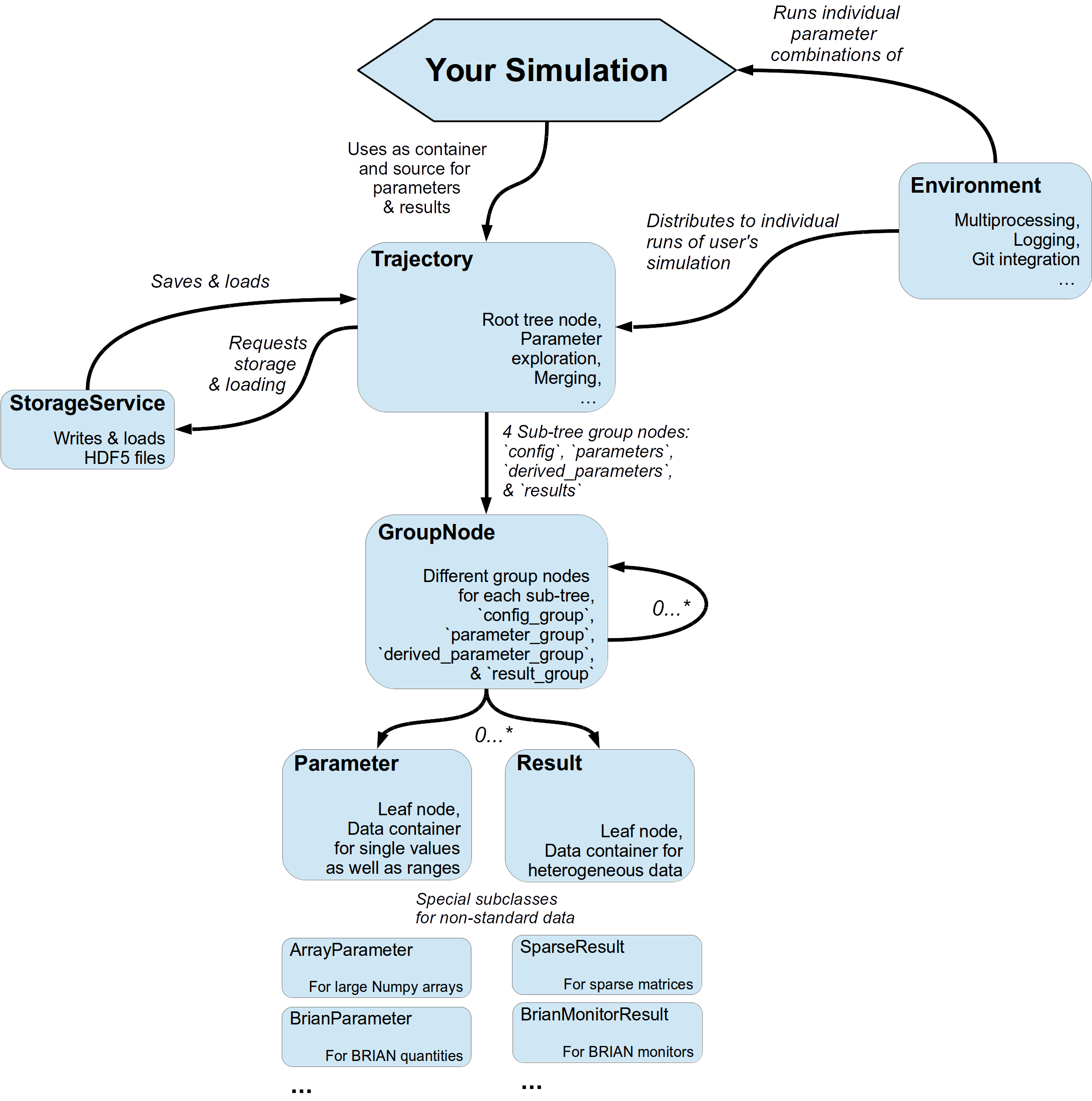
Basic workflow is summarized in the image you can find below. Usually you use an Environment for handling the execution and running of your simulation. As in the example code snippet in the next subsection, the environment will provide a Trajectory container for you to fill in your parameters. During the execution of your simulation with individual parameter combinations, the trajectory can also be used to store results. All data that you hand over to a trajectory is automatically stored into an HDF5 file by the HDF5StorageService.

Quick Working Example¶

The best way to show how stuff works is by giving examples. I will start right away with a very simple code snippet (it can also be found here: First Steps).

Well, what we have in mind is some sort of numerical simulation. For now we will keep it simple, let’s say we need to simulate the multiplication of 2 values, i.e. $z=x*y$ . We have two objectives, a) we want to store results of this simulation $z$ and b) we want to explore the parameter space and try different values of $x$ and $y$ .

Let’s take a look at the snippet at once:

from pypet import Environment, cartesian_product


def multiply(traj):
    """Example of a sophisticated simulation that involves multiplying two values.

    :param traj:

        Trajectory containing
        the parameters in a particular combination,
        it also serves as a container for results.

    """
    z = traj.x * traj.y
    traj.f_add_result('z',z, comment='I am the product of two values!')


# Create an environment that handles running our simulation
env = Environment(trajectory='Multiplication',filename='./HDF/example_01.hdf5',
                  file_title='Example_01',
                  comment='I am a simple example!',
                  large_overview_tables=True)

# Get the trajectory from the environment
traj = env.trajectory

# Add both parameters
traj.f_add_parameter('x', 1.0, comment='Im the first dimension!')
traj.f_add_parameter('y', 1.0, comment='Im the second dimension!')

# Explore the parameters with a cartesian product
traj.f_explore(cartesian_product({'x':[1.0,2.0,3.0,4.0], 'y':[6.0,7.0,8.0]}))

# Run the simulation with all parameter combinations
env.run(multiply)

# Finally disable logging and close all log-files
env.disable_logging()

And now let’s go through it one by one. At first, we have a job to do, that is multiplying two values:

def multiply(traj):
    """Example of a sophisticated simulation that involves multiplying two values.

    :param traj:

        Trajectory containing
        the parameters in a particular combination,
        it also serves as a container for results.

    """
    z=traj.x * traj.y
    traj.f_add_result('z',z, comment='I am the product of two values!')

This is our simulation function multiply. The function makes use of a Trajectory container which manages our parameters. Here the trajectory holds a particular parameter space point, i.e. a particular choice of $x$ and $y$ . In general a trajectory contains many parameter settings, i.e. choices of points sampled from the parameter space. Thus, by sampling points from the space one follows a trajectory through the parameter space - therefore the name of the container.

We can access the parameters simply by natural naming, as seen above via traj.x and traj.y. The value of z is simply added as a result to the traj container.

After the definition of the job that we want to simulate, we create an environment which will run the simulation. Moreover, the environment will take care that the function multiply is called with each choice of parameters once.

# Create an environment that handles running our simulation
env = Environment(trajectory='Multiplication',filename='./HDF/example_01.hdf5',
                  file_title='Example_01',
                  comment = 'I am a simple example!',
                  large_overview_tables=True)

We pass some arguments here to the constructor. This is the name of the new trajectory, a filename to store the trajectory into, the title of the file, and a descriptive comment that is attached to the trajectory. We also set large_overview_tables=True to get a nice summary of all our computed $z$ values in a single table. This is disabled by default to yield smaller and more compact HDF5 files. But for smaller projects with only a few results, you can enable it without wasting much space. You can pass many more (or less) arguments if you like, check out More about the Environment and Environment for a complete list. The environment will automatically generate a trajectory for us which we can access via the property trajectory.

# Get the trajectory from the environment
traj = env.trajectory

Now we need to populate our trajectory with our parameters. They are added with the default values of $x=y=1.0$ .

# Add both parameters
traj.f_add_parameter('x', 1.0, comment='Im the first dimension!')
traj.f_add_parameter('y', 1.0, comment='Im the second dimension!')

Well, calculating $1.0 * 1.0$ is quite boring, we want to figure out more products. Let’s find the results of the cartesian product set $\{1.0, 2.0, 3.0, 4.0\} \times \{6.0, 7.0, 8.0\}$ . Therefore, we use f_explore() in combination with the builder function cartesian_product() that yields the cartesian product of both parameter ranges. You don’t have to explore a cartesian product all the time. You can explore arbitrary trajectories through your space. You only need to pass a dictionary of lists (or other iterables) of the same length with arbitrary entries to f_explore(). In fact, cartesian_product() turns the dictionary {‘x’:[1.0,2.0,3.0,4.0], ‘y’:[6.0,7.0,8.0]} into a new one where the values of ‘x’ and ‘y’ are two lists of length 12 containing all pairings of points.

# Explore the parameters with a cartesian product:
traj.f_explore(cartesian_product({'x':[1.0,2.0,3.0,4.0], 'y':[6.0,7.0,8.0]}))

Finally, we need to tell the environment to run our job multiply with all parameter combinations.

# Run the simulation with all parameter combinations
env.run(multiply)

Usually, if you let pypet manage logging for you, it is a good idea in the end to tell the environment to stop logging and close all log files.

# Finally disable logging and close all log-files
env.disable_logging()

And that’s it. The environment will evoke the function multiply now 12 times with all parameter combinations. Every time it will pass a Trajectory container with another one of these 12 combinations of different $x$ and $y$ values to calculate the value of $z$ . And all of this is automatically stored to disk in HDF5 format.

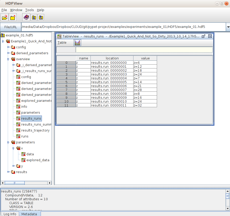
If we now inspect the new HDF5 file in examples/HDF/example_01.hdf5, we can find our trajectory containing all parameters and results. Here you can see the summarizing overview table discussed above.

Loading Data¶

We end this example by showing how we can reload the data that we have computed before. Here we want to load all data at once, but as an example just print the result of run_00000001 where $x$ was 2.0 and $y$ was 6.0. For loading of data we do not need an environment. Instead, we can construct an empty trajectory container and load all data into it by ourselves.

from pypet import Trajectory

# So, first let's create a new empty trajectory and pass it the path and name of the HDF5 file.
traj = Trajectory(filename='experiments/example_01/HDF5/example_01.hdf5')

# Now we want to load all stored data.
traj.f_load(index=-1, load_parameters=2, load_results=2)

# Finally we want to print a result of a particular run.
# Let's take the second run named `run_00000001` (Note that counting starts at 0!).
print('The result of run_00000001 is: ')
print(traj.run_00000001.z)

This yields the statement The result of run_00000001 is: 12 printed to the console.

Some final remarks on the command:

# Now we want to load all stored data.
traj.f_load(index=-1, load_parameters=2, load_results=2)

Above index specifies that we want to load the trajectory with that particular index within the HDF5 file. We could instead also specify a name. Counting works also backwards, so -1 yields the last or newest trajectory in the file.

Next, we need to specify how the data is loaded. Therefore, we have to set the keyword arguments load_parameters and load_results. Here we chose both to be 2.

0 would mean we do not want to load anything at all. 1 would mean we only want to load the empty hulls or skeletons of our parameters or results. Accordingly, we would add parameters or results to our trajectory but they would not contain any data. Instead, 2 means we want to load the parameters and results including the data they contain.

Combining pypet with an Existing Project¶

Of course, you don’t need to start from scratch. If you already have a rather sophisticated simulation environment and simulator, there are ways to integrate or wrap pypet around your project. You may want to look at Combining pypet with an Existing Project and example Wrapping an Existing Project (Cellular Automata Inside!) shows you how to do that.

So that’s it for the start. If you want to know the nitty-gritty details of pypet take a look at the Cookbook (Detailed Manual). If you are not the type of guy who reads manuals but wants hands-on experience, check out the Tutorial or the Examples. If you consider using pypet with an already existing project of yours, I may direct your attention to Wrapping an Existing Project (Cellular Automata Inside!).

Cheers,: Robert