What is pypet all about?
Whenever you do numerical simulations in science, you come across two major problems. First, you need some way to save your data. Secondly, you extensively explore the parameter space. In order to accomplish both you write some hacky IO functionality to get it done the quick and dirty way. Storing stuff into text files, as MATLAB m-files, or whatever comes in handy.
After a while and many simulations later, you want to look back at some of your very first results. But because of unforeseen circumstances, you changed lots of your code. As a consequence, you can no longer use your old data, but you need to write a hacky converter to format your previous results to your new needs. The more complexity you add to your simulations, the worse it gets, and you spend way too much time handling your data and results than doing science.
Indeed, this was a situation I was confronted with pretty quickly during my PhD. So this project was born. I wanted to tackle the IO problems more generally and produce code that was not specific to my current simulations, but I could also use for future scientific projects right out of the box.
The python parameter exploration toolkit (pypet) provides a framework to define parameters that you need to run your simulations. You can actively explore these by following a trajectory through the space spanned by the parameters. And finally, you can get your results together and store everything appropriately to disk. Currently the storage method of choice is HDF5 via PyTables.
Install
Simply install via pip install –pre pypet
Or
Package release can also be found on pypi.python.org. Download, unpack and python setup.py install it.
pypet has been tested for python 2.6 and python 2.7 for Linux using Travis-CI. However, so far there was only limited testing under Windows.
In principle, pypet should work for Windows out of the box if you have installed all prerequisites (pytables, pandas, scipy, numpy). Yet, installing with pip is not possible. You have to download the tar file from pypi.python.org and unzip it (using WinRaR, 7zip, etc. You might need to unpack it twice, first the tar.gz file and then the remaining tar file in the subfolder). Next, open a windows terminal and navigate to your unpacked pypet files to the folder containing the setup.py file. As above run from the terminal python setup.py install.
By the way, the source code is available at github.com/SmokinCaterpillar/pypet.
What to do with pypet?
The whole project evolves around a novel container object called trajectory. A trajectory is a container for parameters and results of numerical simulations in python. In fact a trajectory instantiates a tree and the tree structure will be mapped one to one in the hdf5 file if you store data to disk. But more on that later.
As said before a trajectory contains parameters the basic building blocks that completely define the initial conditions of your numerical simulations. Usually these are very basic data types, like integers, floats or maybe a bit more complex numpy arrays.
For example, you have written a set functions that simulate traffic jam on roads in Rome. Your simulation takes a lot of parameters, the amount of cars (integer), their potential destinations (numpy array of strings), number of pedestrians (integer), random number generator seeds (numpy integer array), open parking spots in Rome (Your parameter is probably None here), and all other sorts of things. These values are added to your trajectory container and can be retrieved from there during the runtime of your simulation.
Doing numerical simulations usually means that you cannot find analytical solutions to your problems. Accordingly, you want to evaluate your simulations on very different parameter settings and investigate the effect of changing the parameters. To phrase that differently, you want to explore the parameter space. Coming back to the traffic jam simulations, you could tell your trajectory that you want to investigate how different amounts of cars and pedestrians influence traffic problems in Rome. So you define sets of combinations of cars and pedestrians and make individual simulation runs for these sets. To phrase that differently, you follow a predefined trajectory of points through your parameter space. And that’s why the container is called trajectory.
For each run of your simulation, with a particular combination of cars and pedestrians, you record time series data of traffic densities at major sites in Rome. This time series data (let’s say they are pandas data frames) can also be added to your trajectory container. In the end everything will be stored to disk. The storage is handled by an extra service to store the trajectory into an HDF5 file on your hard drive. Probably other formats like SQL will come soon (or maybe you want to contribute some code, and write an SQL storage service?).
An example (way less sophisticated than traffic simulations) of a numerical simulation handled by pypet is given below.
Quick (and not so Dirty) Example
The best way to show how stuff works is by giving examples. I will start right away with a very simple code snippet (it can also be found here: 01 First Steps).
Well, what we have in mind is some sort of numerical simulation. For now we will keep it simple, let’s say we need to simulate the multiplication of 2 values, i.e. We have two objectives, a) we want to store results of this simulation and b) we want to explore the parameter space and try different values of and .
Let’s take a look at the snippet at once:
from pypet.environment import Environment
from pypet.utils.explore import cartesian_product


def multiply(traj):
    z=traj.x*traj.y
    traj.f_add_result('z',z=z, comment='Im the product of two reals!')


# Create and environment that handles running
env = Environment(trajectory='Example1_No1',filename='./HDF/example_01.hdf5'',
                  file_title='ExampleNo1', log_folder='./LOGS/',
                  comment='I am a simple example!')

# Get the trajectory from the environment
traj = env.get_trajectory()

# Add both parameters
traj.f_add_parameter('x', 1.0, comment='Im the first dimension!')
traj.f_add_parameter('y', 1.0, comment='Im the second dimension!')

# Explore the parameters with a cartesian product:
traj.f_explore(cartesian_product({'x':[1.0,2.0,3.0,4.0], 'y':[6.0,7.0,8.0]}))

# Run the simulation
env.f_run(multiply)
And now let’s go through it one by one. At first we have a job to do, that is multiplying two real values:
def multiply(traj):
    z=traj.x * traj.y
    traj.f_add_result('z',z=z)
This is our function multiply. The function gets a so called Trajectory container which manages our parameters. We can access the parameters simply by natural naming, as seen above via traj.x and traj.y. The result z is simply added as a result object to the traj container.
After the definition of the job that we want to simulate, we create an environment which will run the simulation.
# Create and environment that handles running
env = Environment(trajectory='Example1_01',filename='./HDF/example_01.hdf5',
                  file_title='Example_01', log_folder='./LOGS/',
                  comment = 'I am a simple example!')
The environment uses some parameters, that is the name of the new trajectory, a filename to store the trajectory into, the title of the file, a folder for the log files, and a comment that is added to the trajectory. The environment will automatically generate a trajectory for us which we can access via:
..code-block::python
# Get the trajectory from the environment traj = env.get_trajectory()
Now we need to populate our trajectory with our parameters. They are added with the default values of
# Add both parameters
traj.f_add_parameter('x', 1.0, comment='Im the first dimension!')
traj.f_add_parameter('y', 1.0, comment='Im the second dimension!')
Well, calculating is quite boring, we want to figure out more products, that is the results of the cartesian product set . Therefore we use f_explore() in combination with the builder function cartesian_product() that yields the cartesian product of both parameters:
# Explore the parameters with a cartesian product:
traj.f_explore(cartesian_product({'x':[1.0,2.0,3.0,4.0], 'y':[6.0,7.0,8.0]}))
Finally, we need to tell the environment to run our job multiply
# Run the simulation
env.f_run(multiply)
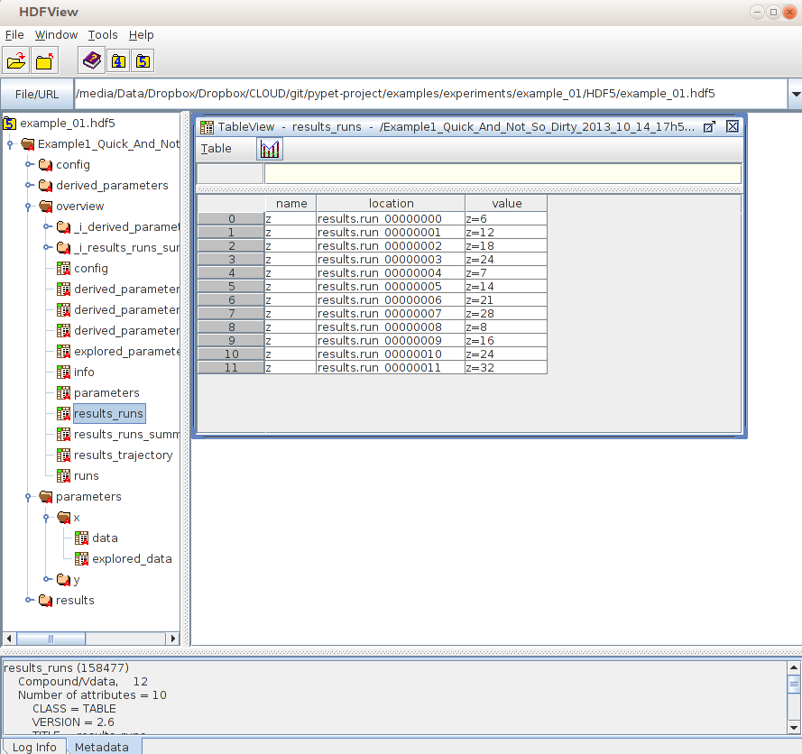
And that’s it. If we now inspect the new hdf5 file in examples/HDF/example_01.hdf5, we will see that our results have been stored right in there, and, of course, the trajectory with our parameters is included, too.
Main Features
Novel tree container Trajectory, for handling and managing of parameters and results of numerical simulations
Grouping of parameters and results
Accessing handled items via natural naming, e.g. traj.parameters.traffic.ncars
Support for many different data formats
Easily extendible to other data formats!
Exploration of the parameter space of your simulations
Merging of trajectories residing in the same space
Support for multiprocessing, distribute your individual simulation runs to several processes.
Storage of simulation data, i.e. the trajectory, parameters, and results into HDF5 files
Dynamic Loading, load only the data you need at the moment and free it afterwards
Resuming a crashed simulation (maybe due to power shut down) after the latest completed run
Annotations of parameters, results and groups, these annotations are stored as HDF5 node attributes
Git Integration, make automatic commits of your source code every time you run an experiment