Tutorial¶

Conceptualization of a Numerical Experiment¶

I will give a simple but comprehensive tutorial on pypet and how to use it for parameter exploration of numerical experiments in python.

pypet is designed to support your numerical simulations in two ways: Allow a) easy exploration of the parameter space of your simulations and b) easy storage of the results.

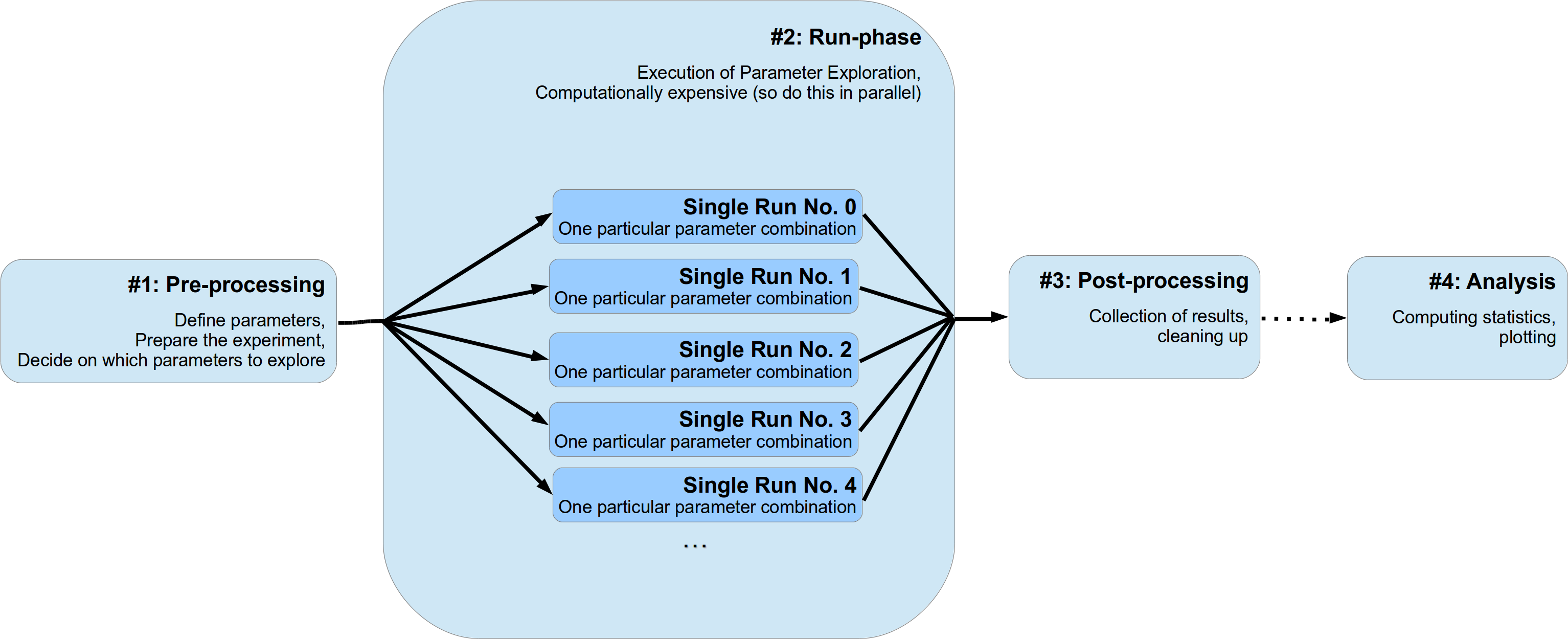
We will assume that usually a numerical experiments consist of two to four different stages:

Pre-processing

Parameter definition, preparation of the experiment

The run phase of your experiment

Fan-out structure, usually parallel running of different parameter settings, gathering of individual results for each single run

Post-processing (optional)

Cleaning up of the experiment, sorting results, etc.

Analysis of results (optional)

Plotting, doing statistics etc.

The first stage can be further divided into two sub-stages. In the beginning the definition of parameters (either directly in the source code or by parsing a configuration file) and, next, the appropriate setup of your experiment. This might involve creating particular python objects or pre-computing some expensive functions etc. Moreover, here you also decide if you want to deviate from your default set of parameters and explore the parameter space and try a bunch of different settings. Probably you want to do a sensitivity analysis and determine the effect of changing a critical subset of your parameters.

The second stage, the run phase, is the actual execution of your numerical simulation. Here you perform the search or exploration of the parameter space. You try all different parameter settings you have specified before for exploration and obtain the corresponding results. Since this stage is most likely the computational expensive one, you probably want to parallelize your simulations. I will refer to an individual simulation run with one particular parameter combination as a single run of your simulation. Since these single runs are different individual simulations with different parameter settings, they are completely independent of each other. The results and outcomes of one single run should not influence another. Sticking to this assumption makes the parallelization of your experiments much easier. This doesn’t mean that non-independent runs cannot be handled by pypet (they can!), it rather means you should not do this for cleaner and easier portable code and simulations.

Thirdly, after all individual single runs are completed you might have a phase of post-processing. This could encompass merging or collecting of results of individual single runs and/or deconstructing some sensitive python objects, etc.

Finally, you do further analysis of the raw results of your numerical simulation, like generating plots and meta statistics, etc. Personally, I would strictly separate this final phase from the previous three. Thus, using a complete different python script than for the phases before.

This conceptualization is depicted in the figure below:

pypet gives is you a tool to make the stages much easier to handle. pypet offers a novel tree data container called Trajectory that can be used to store all parameters and results of your numerical simulations. Moreover, pypet has an Environment that allows easy parallel exploration of the parameter space.

We will see how we can use both in our numerical experiment at the different stages. In this tutorial we will simulate a simple neuron model, called leaky integrate-and-fire model. Our neuron model is given by a dynamical variable $V$ that describes the development of the so called membrane potential over time. Every time this potential crosses a particular threshold our neuron is activated and emits an electrical pulse. These pules, called action potentials or spikes, are the sources of information transmission in the brain. We will stimulate our neuron with an experimental current $I$ and see how this current affects the emission of spikes. For simplicity we assume a system without any physical units except for time in milliseconds.

We will numerically integrate the linear differential equation:

$\frac{dV}{dt} = -\frac{1}{\tau_V} V + I$

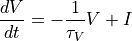
with a non-linear reset rule $V \leftarrow 0$ if $V \geq 1$ and an additional refractory period of $\tau_{ref}$ . If we detect an action potential, i.e. $V \geq 1$ , we will keep the voltage $V$ clamped to 0 for the refractory period after the threshold crossing and freeze the differential equation.

Regarding parameter exploration, we will hold the neuron’s time constant $\frac{1}{\tau_V}=10$ ms fixed and explore the parameter space by varying different input currents $I$ and different lengths of the refractory period $\tau_{ref}$ .

During the single runs we will record the development of the variable $V$ over time and count the number of threshold crossings to estimate the so called firing rate of a neuron. In the post processing phase we will collect these firing rates and write them into a pandas DataFrame. Don’t worry if you are not familiar with pandas. Basically, a pandas DataFrame instantiates a table. It’s like a 2D numpy array, but we can index into the table by more than just integers.

Finally, during the analysis, we will plot the neuron’s rate as a function of the input current $I$ and the refractory period $\tau_{ref}$ .

The entire source code of this example can be found here: Post-Processing and Pipelining (from the Tutorial).

Naming Convention¶

To avoid confusion with natural naming scheme and the functionality provided by the trajectory tree - that includes all group and leaf nodes like parameters and results - I followed the idea by PyTables to use prefixes: f_ for functions and v_ for python variables/attributes/properties.

For instance, given a pypet result container myresult, myresult.v_comment is the object’s comment attribute and myresult.f_set(mydata=42) is the function for adding data to the result container. Whereas myresult.mydata might refer to a data item named mydata added by the user.

If you don’t like using prefixes, you can alternatively also use the properties vars and func that are supported by each tree node. For example, traj.f_iter_runs() is equivalent to traj.func.iter_runs() or mygroup.v_full_name is equivalent to mygroup.vars.full_name.

The prefix and vars/func notation only applies to tree data objects (group nodes and leaf nodes) but not to other aspects of pypet. For example, the Environment does not rely on prefixes at all.

#1 Pre-Processing¶

Your experiment usually starts with the creation of an Environment. Don’t worry about the huge amount of parameters you can pass to the constructor, these are more for tweaking of your experiment and the default settings are usually suitable.

Yet, we will shortly discuss the most important ones here.

trajectory

Here you can either pass an already existing trajectory container or simply a string specifying the name of a new trajectory. In the latter case the environment will create a trajectory container for you.
add_time

If True and the environment creates a new trajectory container, it will add the current time to the name in the format _XXXX_XX_XX_XXhXXmXXs. So for instance, if you set trajectory='Gigawatts_Experiment' and add_time=true, your trajectory’s name will be Gigawatts_Experiment_2015_10_21_04h23m00s.
comment

A nice descriptive comment about what you are going to do in your numerical experiment.
log_config

The name of a logging .ini file specifying the logging set up. See Logging, or the logging documentation and how to specify logging config files. If set to DEFAULT_LOGGING ('DEFAULT') the default settings are used. Simply set to None if you want to disable logging.
multiproc

If we want to use multiprocessing. We sure do so, so we set this to True.
ncores

The number of cpu cores we want to utilize. More precisely, the number of processes we start at the same time to calculate the single runs. There’s usually no benefit in setting this value higher than the actual number of cores your computer has.
filename

We can specify the name of the resulting HDF5 file where all data will be stored. We don’t have to give a filename per se, we can also specify a folder './results/' and the new file will have the name of the trajectory.
git_repository

If your code base is under git version control (it’s not? Stop reading and get git NOW! ;-), you can specify the path to your root git folder here. If you do this, pypet will a) trigger a new commit if it detects changes in the working copy of your code and b) write the corresponding commit code into your trajectory so you can immediately see with which version you did your experiments.
git_fail

If you don’t want automatic commits, simply set git_fail=True. Given changes in your code base, your program will throw a GitDiffError instead of making an automatic commit. Then, you can manually make a commit and restart your program with the committed changes.
sumatra_project

If your experiments are recorded with sumatra you can specify the path to your sumatra root folder here. pypet will automatically trigger the recording of your experiments if you use run(), resume() or pipeline() to start your single runs or whole experiment. If you use pypet + git + sumatra there’s no doubt that you ensure the repeatability of your experiments!

Ok, so let’s start with creating an environment:

from pypet import Environment
env = Environment(trajectory='FiringRate',
                  comment='Experiment to measure the firing rate '
                        'of a leaky integrate and fire neuron. '
                        'Exploring different input currents, '
                        'as well as refractory periods',
                  add_time=False, # We don't want to add the current time to the name,
                  log_config='DEFAULT',
                  multiproc=True,
                  ncores=2, # My laptop has 2 cores ;-)
                  filename='./hdf5/', # We only pass a folder here, so the name is chosen
                  # automatically to be the same as the Trajectory
                  )

The environment provides a new trajectory container for us:

traj = env.trajectory

The Trajectory Container¶

A Trajectory is the container for your parameters and results. It basically instantiates a tree.

This tree has four major branches: config (parameters), parameters, derived_parameters and results.

Parameters stored under config do not specify the outcome of your simulations but only the way how the simulations are carried out. For instance, this might encompass the number of cpu cores for multiprocessing. In fact, the environment from above has already added the config data we specified before to the trajectory:

>>> traj.config.ncores
2

Parameters in the parameters branch are the fundamental building blocks of your simulations. Changing a parameter usually effects the results you obtain in the end. The set of parameters should be complete and sufficient to characterize a simulation. Running a numerical simulation twice with the very same parameter settings should give also the very same results. So make sure to also add seed values of random number generators to your parameter set.

Derived parameters are specifications of your simulations that, as the name says, depend on your original parameters but are still used to carry out your simulation. They are somewhat too premature to be considered as final results. We won’t have any of these in the tutorial so you can ignore this branch for the moment.

Anything found under results is, as expected, a result of your numerical simulation.

Adding of Parameters¶

Ok, for the moment let’s fill the trajectory with parameters for our simulation.

Let’s fill it using the f_add_parameter() function:

traj.f_add_parameter('neuron.V_init', 0.0,
                     comment='The initial condition for the '
                                'membrane potential')
traj.f_add_parameter('neuron.I', 0.0,
                     comment='The externally applied current.')
traj.f_add_parameter('neuron.tau_V', 10.0,
                     comment='The membrane time constant in milliseconds')
traj.f_add_parameter('neuron.tau_ref', 5.0,
                    comment='The refractory period in milliseconds '
                            'where the membrane potnetial '
                            'is clamped.')

traj.f_add_parameter('simulation.duration', 1000.0,
                     comment='The duration of the experiment in '
                            'milliseconds.')
traj.f_add_parameter('simulation.dt', 0.1,
                     comment='The step size of an Euler integration step.')

Again we can provide descriptive comments. All these parameters will be added to the branch parameters.

As a side remark, if you think there’s a bit too much typing involved here, you can also make use of much shorter notations. For example, granted you imported the Parameter, you could replace the last addition by:

traj.parameters.simulation.dt = Parameter('dt', 0.1, comment='The step size of an Euler integration step.')

Or even shorter:

traj.par.simulation.dt = 0.1, 'The step size of an Euler integration step.'

Note that we can group the parameters. For instance, we have a group neuron that contains parameters defining our neuron model and a group simulation that defines the details of the simulation, like the euler step size and the whole runtime. If a group does not exist at the time of a parameter creation, pypet will automatically create the groups on the fly.

There’s no limit to grouping, and it can be nested:

>>> traj.f_add_parameter('brian.hippocampus.nneurons', 99999, comment='Number of neurons in my model hippocampus')

There are analogue functions for config data, results and derived_parameters:

If you don’t want to stick to these four major branches there is the generic addition:

f_add_leaf()

By the way, you can add particular groups directly with:

and the generic one:

f_add_group()

Your trajectory tree contains two types of nodes, group nodes and leaf nodes. Group nodes can, as you have seen, contain other group or leaf nodes, whereas leaf nodes are terminal and do not contain more groups or leaves.

The leaf nodes are abstract containers for your actual data. Basically, there exist two sub-types of these leaves Parameter containers for your config data, parameters, and derived parameters and Result containers for your results.

A Parameter can only contain a single data item plus potentially a range or list of different values describing how the parameter should be explored in different runs.

A Result container can manage several results. You can think of it as non-nested dictionary. Actual data can also be accessed via natural naming or squared brackets (as discussed in the next section below).

For instance:

>>> traj.f_add_result('deep.thought', answer=42, question='What do you get if you multiply six by nine?')
>>> traj.results.deep.thought.question
'What do you get if you multiply six by nine?'

Both leaf containers (Parameter, Result) support a rich variety of data types. There also exist more specialized versions if the standard ones cannot hold your data, just take a look at More on Parameters and Results. If you are still missing some functionality for your particular needs you can simply implement your own leaf containers and put them into the trajectory.

Accessing Data¶

Data can be accessed in several ways. You can, for instance, access data via natural naming: traj.parameters.neuron.tau_ref or square brackets traj['parameters']['neuron']['tau_ref'] or traj['parameters.neuron.tau_ref'], or traj['parameters','neuron','tau_ref'], or use the f_get() method.

As long as your tree nodes are unique, you can shortcut through the tree. If there’s only one parameter tau_ref, traj.tau_ref is equivalent to traj.parameters.neuron.tau_ref.

Moreover, since a Parameter only contains a single value (apart from the range), pypet will assume that you usually don’t care about the actual container but just about the data. Thus, traj.parameters.neuron.tau_ref will immediately return the data value for tau_ref and not the corresponding Parameter container. If you really need the container itself use f_get(). To learn more about this concept of fast access of data look at Accessing Data in the Trajectory.

Exploring the Data¶

Next, we can tell the trajectory which parameters we want to explore. We simply need need to pass a dictionary of lists (or other iterables) of the same length with arbitrary entries to the trajectory function f_explore().

Every single run in the run phase will contain one setting of parameters in the list. For instance, if our exploration dictionary looks like {'x':[1,2,3], 'y':[1,1,2]} the first run will be with parameter x set to 1 and y to 1, the second with x set to 2 and y set to 1, and the final third one with x=3 and y=2.

If you want to explore the cartesion product of two iterables not having the same length you can use the cartesian_product() builder function. This will return a dictionary of lists of the same length and all combinations of the parameters.

Here is our exploration, we try unitless currents $I$ ranging from 0 to 1.01 in steps of 0.01 for three different refractory periods $\tau_{ref}$ :

from pypet.utils.explore import cartesian_product

explore_dict = {'neuron.I': np.arange(0, 1.01, 0.01).tolist(),
                'neuron.tau_ref': [5.0, 7.5, 10.0]}

explore_dict = cartesian_product(explore_dict, ('neuron.tau_ref', 'neuron.I'))
# The second argument, the tuple, specifies the order of the cartesian product,
# The variable on the right most side changes fastest and defines the
# 'inner for-loop' of the cartesian product

traj.f_explore(explore_dict)

Note that in case we explore some parameters, their default values that we passed before via f_add_parameter() are no longer used. If you still want to simulate these, make sure they are part of the lists in the exploration dictionary.

#2 The Run Phase¶

Next, we define a job or top-level simulation run function (that not necessarily has to be a real python function, any callable object will do the job). This function will be called and executed with every parameter combination we specified before with f_explore() in the trajectory container.

In our neuron simulation we have 303 different runs of our simulation. Each run has particular index ranging from 0 to 302 and a particular name that follows the structure run_XXXXXXXX where XXXXXXXX is replaced with the index and some leading zeros. Thus, our run names range from run_00000000 to run_00000302.

Note that we start counting with 0, so the second run is called run_00000001 and has index 1!

So here is our top-level simulation or run function:

def run_neuron(traj):
    """Runs a simulation of a model neuron.

    :param traj:

        Container with all parameters.

    :return:

        An estimate of the firing rate of the neuron

    """

    # Extract all parameters from `traj`
    V_init = traj.par.neuron.V_init
    I = traj.par.neuron.I
    tau_V = traj.par.neuron.tau_V
    tau_ref = traj.par.neuron.tau_ref
    dt = traj.par.simulation.dt
    duration = traj.par.simulation.duration

    steps = int(duration / float(dt))
    # Create some containers for the Euler integration
    V_array = np.zeros(steps)
    V_array[0] = V_init
    spiketimes = []  # List to collect all times of action potentials

    # Do the Euler integration:
    print('Starting Euler Integration')
    for step in range(1, steps):
        if V_array[step-1] >= 1:
            # The membrane potential crossed the threshold and we mark this as
            # an action potential
            V_array[step] = 0
            spiketimes.append((step-1)*dt)
        elif spiketimes and step * dt - spiketimes[-1] <= tau_ref:
            # We are in the refractory period, so we simply clamp the voltage
            # to 0
            V_array[step] = 0
        else:
            # Euler Integration step:
            dV = -1/tau_V * V_array[step-1] + I
            V_array[step] = V_array[step-1] + dV*dt

    print('Finished Euler Integration')

    # Add the voltage trace and spike times
    traj.f_add_result('neuron.$', V=V_array, nspikes=len(spiketimes),
                  comment='Contains the development of the membrane potential over time '
                          'as well as the number of spikes.')
    # This result will be renamed to `traj.results.neuron.run_XXXXXXXX`.


    # And finally we return the estimate of the firing rate
    return len(spiketimes) / float(traj.par.simulation.duration) * 1000
    # *1000 since we have defined duration in terms of milliseconds

Our function has to accept at least one argument and this is our traj container. During the execution of our simulation function the trajectory will contain just one parameter setting out of our 303 different ones from above. The environment will make sure that our function is called with each of our parameter choices once.

For instance, if we currently execute the second run (aka run_00000001) all parameters will contain their default values, except tau_ref and I, they will be set to 5.0 and 0.01, respectively.

Let’s take a look at the first few instructions:

# Extract all parameters from `traj`
V_init = traj.par.neuron.V_init
I = traj.par.neuron.I
tau_V = traj.par.neuron.tau_V
tau_ref = traj.par.neuron.tau_ref
dt = traj.par.simulation.dt
duration = traj.par.simulation.duration

So here we simply extract the parameter values from traj. As said before pypet is smart to directly return the data value instead of a Parameter container. Moreover, remember all parameters will have their default values except tau_ref and I.

Next, we create a numpy array and a python list and compute the number of steps. This is not specific to pypet but simply needed for our neuron simulation:

steps = int(duration / float(dt))
# Create some containers for the Euler integration
V_array = np.zeros(steps)
V_array[0] = V_init
spiketimes = []  # List to collect all times of action potentials

Also the following steps have nothing to do with pypet, so don’t worry if you not fully understand what’s going on here. This is just the core of our neuron simulation:

# Do the Euler integration:
print('Starting Euler Integration')
for step in range(1, steps):
    if V_array[step-1] >= 1:
        # The membrane potential crossed the threshold and we mark this as
        # an action potential
        V_array[step] = 0
        spiketimes.append((step-1)*dt)
    elif spiketimes and step * dt - spiketimes[-1] <= tau_ref:
        # We are in the refractory period, so we simply clamp the voltage
        # to 0
        V_array[step] = 0
    else:
        # Euler Integration step:
        dV = -1/tau_V * V_array[step-1] + I
        V_array[step] = V_array[step-1] + dV*dt

print('Finished Euler Integration')

This is simply the python description of the following set of equations:

$\frac{dV}{dt} = -\frac{1}{\tau_V} V + I$

and $V \leftarrow 0$ if $V \geq 1$ or $t-t_{s} \leq \tau_{ref}$ (with $t$ the current time and $t_{s}$ time of the last spike).

Ok, for now we have finished one particular run ouf our simulation. We computed the development of the membrane potential $V$ over time and put it into V_array.

Next, we hand over this data to our trajectory, since we want to keep it and write it into the final HDF5 file:

traj.f_add_result('neuron.$', V=V_array, nspikes=len(spiketimes),
                  comment='Contains the development of the membrane potential over time '
                          'as well as the number of spikes.')

This statement looks similar to the addition of parameters we have seen before. Yet, there are some subtle differences. As we can see, a result can contain several data items. If we pass them via NAME=value, we can later on recall them from the result with result.NAME. Secondly, there is this odd '$' character in the result’s name. Well, recall that we are currently operating in the run phase, accordingly the run_neuron function will be executed many times. Thus, we also gather the V_array data many times. We need to store this every time under a different name in our trajectory tree. '$' is a wildcard character that is replaced by the name of the current run. If we were in the second run, we would store everything under traj.results.neuron.run_00000001 and in the third run under traj.results.neuron.run_00000002 and so on and so forth. Consequently, calling traj.results.neuron.run_00000001.V will return our membrane voltage array of the second run.

You are not limited to place the '$' at the end, for example

traj.f_add_result('fundamental.wisdom.$.answer', 42, comment='The answer')

would be possible as well.

As a side remark, if you add a result or derived parameter during the run phase but not use the '$' wildcard, pypet will add runs.'$' to the beginning of your result’s or derived parameter’s name.

So executing the following statement during the run phase

traj.f_add_result('fundamental.wisdom.answer', 42, comment='The answer')

will yield a renaming to results.runs.run_XXXXXXXXX.fundamental.wisdom.answer. Where run_XXXXXXXXX is the name of the corresponding run, of course.

Moreover, it’s worth noticing that you don’t have to explicitly write the trajectory to disk. Everything you add during pre-processing, post-processing (see below) is automatically stored at the end of the experiment. Everything you add during the run phase under a group or leaf node called run_XXXXXXXX (where this is the name of the current run, which will be automatically chosen if you use the '$' wildcard) will be stored at the end of the particular run.

#3 Post-Processing¶

Each single run of our run_neuron function returned an estimate of the firing rate. In the post processing phase we want to collect these estimates and sort them into a table according to the value of $I$ and $\tau_{ref}$ . As an appropriate table we choose a pandas DataFrame. Again this is not pypet specific but pandas offers neat containers for series, tables and multidimensional panel data. The nice thing about pandas containers is that they except all forms of indices and not only integer indices like python lists or numpy arrays.

So here comes our post processing function. This function will be automatically called when all single runs are completed. The post-processing function has to take at least two arguments. First one is the trajectory, second one is the list of results. This list actually contains two-dimensional tuples. First entry of the tuple is the index of the run as an integer, and second entry is the result returned by our job-function run_neuron in the corresponding run.

def neuron_postproc(traj, result_list):
    """Postprocessing, sorts firing rates into a data frame.

    :param traj:

        Container for results and parameters

    :param result_list:

        List of tuples, where first entry is the run index and second is the actual
        result of the corresponding run.

    :return:
    """

    # Let's create a pandas DataFrame to sort the computed firing rate according to the
    # parameters. We could have also used a 2D numpy array.
    # But a pandas DataFrame has the advantage that we can index into directly with
    # the parameter values without translating these into integer indices.
    I_range = traj.par.neuron.f_get('I').f_get_range()
    ref_range = traj.par.neuron.f_get('tau_ref').f_get_range()

    I_index = sorted(set(I_range))
    ref_index = sorted(set(ref_range))
    rates_frame = pd.DataFrame(columns=ref_index, index=I_index)
    # This frame is basically a two dimensional table that we can index with our
    # parameters

    # Now iterate over the results. The result list is a list of tuples, with the
    # run index at first position and our result at the second
    for result_tuple in result_list:
        run_idx = result_tuple[0]
        firing_rates = result_tuple[1]
        I_val = I_range[run_idx]
        ref_val = ref_range[run_idx]
        rates_frame.loc[I_val, ref_val] = firing_rates # Put the firing rate into the
        # data frame

    # Finally we going to store our new firing rate table into the trajectory
    traj.f_add_result('summary.firing_rates', rates_frame=rates_frame,
                      comment='Contains a pandas data frame with all firing rates.')

Ok, we will go through it one by one. At first we extract the range of parameters we used:

I_range = traj.par.neuron.f_get('I').f_get_range()
ref_range = traj.par.neuron.f_get('tau_ref').f_get_range()

Note that we use pypet.naturalnaming.NNGroupNode.f_get() here since we are interested in the parameter container not the data value. We can directly extract the parameter range from the container via $pypet.parameter.Parameter.f_get_range$ .

Next, we create a two dimensional table aka pandas DataFrame with the current as the row indices and the refractory period as column indices.

I_index = sorted(set(I_range))
ref_index = sorted(set(ref_range))
rates_frame = pd.DataFrame(columns=ref_index, index=I_index)

Now we iterate through the result tuples and write the firing rates into the table according to the parameter settings in this run. As said before, the nice thing about pandas is that we can use the values of $I$ and $\tau_{ref}$ as indices for our table.

for result_tuple in result_list:
        run_idx = result_tuple[0]
        firing_rates = result_tuple[1]
        I_val = I_range[run_idx]
        ref_val = ref_range[run_idx]
        rates_frame.loc[I_val, ref_val] = firing_rates

Finally, we add the filled DataFrame to the trajectory.

traj.f_add_result('summary.firing_rates', rates_frame=rates_frame,
                      comment='Contains a pandas data frame with all firing rates.')

Since we are no longer in the run phase, this result will be found in traj.results.summary.firing_rate and no name of any single run will be added.

This was our post-processing where we simply collected all firing rates and sorted them into a table. You can, of course, do much more in the post processing phase. You can load all computed data and look at it. You can even expand the trajectory to trigger a new run phase. Accordingly, you can adaptively and iteratively search the parameter space. You may even do this on the fly while there are still single runs being executed, see Adding Post-Processing.

Final Steps in the Main Script¶

Still we actually need to make the environment execute all the stuff, so this is our main script after we generated the environment and added the parameters. First, we add the post-processing function. Secondly, we tell the environment to run our function run_neuron. Our postprocessing function will be automatically called after all runs have finished.

# Ad the postprocessing function
env.add_postprocessing(neuron_postproc)

# Run the experiment
env.run(run_neuron)

Both function take additional arguments which will be automatically passed to the job and post-processing functions.

For instance,

env.run(myjob, 42, 'fortytwo', test=33.3)

will additionally pass 42, 'fortytwo' as positional arguments and test=33.3 as the keyword argument test to your run function. So the definition of the run function could look like this:

def myjob(traj, number, text, test):
    # do something

Remember that the trajectory will always be passed as first argument. This works analogously for the post-processing function as well. Yet, there is the slight difference that your post-processing function needs to accept the result list as second positional argument followed by your positional and keyword arguments.

Finally, if you used pypet’s logging feature, it is usually a good idea to tell the environment to stop logging and close all log files:

# Finally disable logging and close all log-files
env.disable_logging()

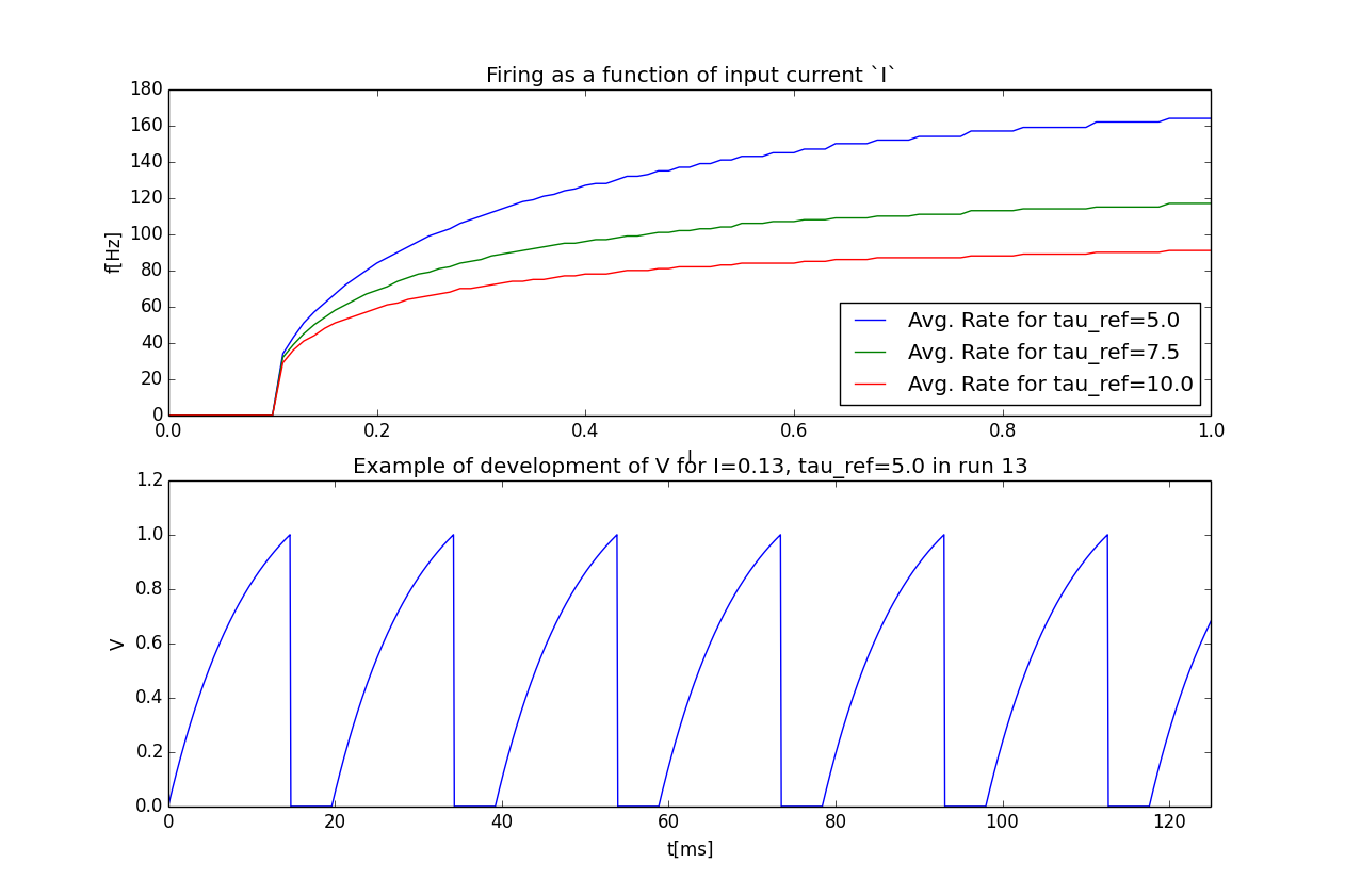
#4 Analysis¶

The final stage of our experiment encompasses the analysis of our raw data. We won’t do much here, simply plot our firing rate table and show one example voltage trace. All data analysis happens in a completely different script and is executed independently of the previous three steps except that we need the data from them in form of a trajectory.

We will make use of the Automatic Loading functionality and load results in the background as we need them. Since we don’t want to do any more single runs, we can spare us an environment and only use a trajectory container.

from pypet import Trajectory
import matplotlib.pyplot as plt

# This time we don't need an environment since we just going to look
# at data in the trajectory
traj = Trajectory('FiringRate', add_time=False)

# Let's load the trajectory from the file
# Only load the parameters, we will load the results on the fly as we need them
traj.f_load(filename='./hdf5/FiringRate.hdf5', load_parameters=2,
            load_results=0, load_derived_parameters=0)

# We'll simply use auto loading so all data will be loaded when needed.
traj.v_auto_load = True

# Here we load the data automatically on the fly
rates_frame = traj.res.summary.firing_rates.rates_frame

plt.figure()
plt.subplot(2,1,1)
#Let's iterate through the columns and plot the different firing rates :
for tau_ref, I_col in rates_frame.iteritems():
    plt.plot(I_col.index, I_col, label='Avg. Rate for tau_ref=%s' % str(tau_ref))

# Label the plot
plt.xlabel('I')
plt.ylabel('f[Hz]')
plt.title('Firing as a function of input current `I`')
plt.legend()

# Also let's plot an example run, how about run 13?
example_run = 13

traj.v_idx = example_run # We make the trajectory behave as a single run container.
# This short statement has two major effects:
# a) all explored parameters are set to the value of run 13,
# b) if there are tree nodes with names other than the current run aka `run_00000013`
# they are simply ignored, if we use the `$` sign or the `crun` statement,
# these are translated into `run_00000013`.

# Get the example data
example_I = traj.I
example_tau_ref = traj.tau_ref
example_V = traj.results.neuron.crun.V # Here crun stands for run_00000013

# We need the time step...
dt = traj.dt
# ...to create an x-axis for the plot
dt_array = [irun * dt for irun in range(len(example_V))]

# And plot the development of V over time,
# Since this is rather repetitive, we only
# plot the first eighth of it.
plt.subplot(2,1,2)
plt.plot(dt_array, example_V)
plt.xlim((0, dt*len(example_V)/8))

# Label the axis
plt.xlabel('t[ms]')
plt.ylabel('V')
plt.title('Example of development of V for I=%s, tau_ref=%s in run %d' %
          (str(example_I), str(example_tau_ref), traj.v_idx))

# And let's take a look at it
plt.show()

# Finally revoke the `traj.v_idx=13` statement and set everything back to normal.
# Since our analysis is done here, we could skip that, but it is always a good idea
# to do that.
traj.f_restore_default()

The outcome of your little experiment should be the following image:

Finally, I just want to make some final remarks on the analysis script.

traj.f_load(filename='./hdf5/FiringRate.hdf5', load_parameters=2,
            load_results=0, load_derived_parameters=0)

describes how the different subtrees of the trajectory are loaded (load_parameters also includes the config branch). 0 means no data at all is loaded, 1 means only the containers are loaded but without any data and 2 means the containers including the data are loaded. So here we load all parameters and all config parameters with data and no results whatsoever.

Yet, since we say traj.v_auto_load = True the statement rates_frame = traj.res.summary.firing_rates.rates_frame will return our 2D table of firing rates because the data is loaded in the background while we request it.

Furthermore,

traj.v_idx = example_run

is an important statement in the code. Setting the properties v_idx or v_crun or using the function f_set_crun() are equivalent. These give you a powerful tool in data analysis because they make your trajectory behave like a particular single run. Thus, all explored parameter’s values will be set to the corresponding values of one particular run.

To restore everything back to normal simply call f_restore_default().

This concludes our small tutorial. If you are interested in more advance concepts look into the cookbook or check out the code snippets in the example section. Notably, if you consider using pypet with an already existing project of yours, you might want to pay attention to Wrapping an Existing Project (Cellular Automata Inside!) and Combining pypet with an Existing Project.

Cheers,: Robert